|
Basics of Radio Astronomy - Goldstone-Apple Valley Radio Telescope
(GAVRT):
This is a JPL Presentation of the basics of radio astronomy. This is an ASP
version of the
original PDF
on-line book.
Back to
Astronomy Tools
Basics of Radio Astronomy
for the
Goldstone-Apple Valley
Radio Telescope
Prepared by
Diane Fisher Miller
Advanced Mission Operations Section
Also available on the Internet at URL
http://www.jpl.nasa.gov/radioastronomy
April 1998
JPL D-13835
Table of Contents:
Back to Top |
Back to
Astronomy Tools
Preface -
Back to Table of Contents
In a collaborative effort, the Science and Technology Center (in Apple Valley,
California), the
Apple Valley Unified School District, the Jet Propulsion Laboratory, and NASA
have converted a
34-meter antenna at NASA's Deep Space Network's Goldstone Complex into a unique
interactive
research and teaching instrument available to classrooms throughout the United
States, via the
Internet. The Science and Technology Center is a branch of the Lewis Center for
Educational
Research.
The Goldstone-Apple Valley Radio Telescope (GAVRT) is located in a remote area
of the
Mojave Desert, 40 miles north of Barstow, California. The antenna, identified as
DSS-12, is a 34-
meter diameter dish, 11 times the diameter of a ten-foot microwave dish used for
satellite television
reception. DSS-12 has been used by NASA to communicate with robotic space probes
for
more than thirty years. In 1994, when NASA decided to decommission DSS-12 from
its operational
network, a group of professional scientists, educators, engineers, and several
community
volunteers envisioned a use for this antenna and began work on what has become
the GAVRT
Project.
The GAVRT Project is jointly managed by the Science and Technology Center and
the DSN
Science Office, Telecommunications and Mission Operations Directorate, at the
Jet Propulsion
Laboratory.
This workbook was developed as part of the training of teachers and volunteers
who will be
operating the telescope. The students plan observations and operate the
telescope from the Apple
Valley location using Sun workstations. In addition, students and teachers in
potentially 10,000
classrooms across the country will be able to register with the center’s Web
site and operate the
telescope from their own classrooms.
Introduction -
Back to Table of Contents
This module is the first in a sequence to prepare volunteers and teachers at the
Science and
Technology Center to operate the Goldstone-Apple Valley Radio Telescope (GAVRT).
It covers
the basic science concepts that will not only be used in operating the
telescope, but that will make
the experience meaningful and provide a foundation for interpreting results.
Acknowledgements -
Back to Table of Contents
Many people contributed to this workbook. The first problem we faced was to
decide which of
the overwhelming number of astronomy topics we should cover and at what depth in
order to
prepare GAVRT operators for the radio astronomy projects they would likely be
performing.
George Stephan generated this initial list of topics, giving us a concrete
foundation on which to
begin to build. Thanks to the subject matter experts in radio astronomy, general
astronomy, and
physics who patiently reviewed the first several drafts and took time to explain
some complex
subjects in plain English for use in this workbook. These kind reviewers are Dr.
M.J. Mahoney,
Roger Linfield, David Doody, Robert Troy, and Dr. Kevin Miller (who also loaned
the project
several most valuable books from his personal library). Special credit goes to
Dr. Steve Levin,
who took responsibility for making sure the topics covered were the right ones
and that no known
inaccuracies or ambiguities remained. Other reviewers who contributed
suggestions for clarity
and completeness were Ben Toyoshima, Steve Licata, Kevin Williams, and George
Stephan.
Assumptions and Disclaimers -
Back to Table of Contents
This training module assumes you have an understanding of high-school-level
chemistry, physics,
and algebra. It also assumes you have familiarity with or access to other
materials on general
astronomy concepts, since the focus here is on those aspects of astronomy that
relate most
specifically to radio astronomy.
This workbook does not purport to cover its selected topics in depth, but simply
to introduce them
and provide some context within the overall disciplines of astronomy in general
and radio astronomy
in particular. It does not cover radio telescope technology, nor details of
radio astronomy
data analysis.
Back to Top |
Back to
Astronomy Tools
Chapter 1 -
Back to Table of Contents
Overview: Discovering an Invisible Universe
Objectives: Upon completion of this chapter, you will be able to describe the
general principles
upon which radio telescopes work.
Before 1931, to study astronomy meant to study the objects visible in the night
sky. Indeed, most
people probably still think that’s what astronomers do—wait until dark and look
at the sky using
their naked eyes, binoculars, and optical telescopes, small and large. Before
1931, we had no
idea that there was any other way to observe the universe beyond our atmosphere.
In 1931, we did know about the electromagnetic spectrum. We knew that visible
light included
only a small range of wavelengths and frequencies of energy. We knew about
wavelengths
shorter than visible light—Wilhelm Röntgen had built a machine that produced
x-rays in 1895.
We knew of a range of wavelengths longer than visible light (infrared), which in
some circumstances
is felt as heat. We even knew about radio frequency (RF) radiation, and had been
developing
radio, television, and telephone technology since Heinrich Hertz first produced
radio waves
of a few centimeters long in 1888. But, in 1931, no one knew that RF radiation
is also emitted by
billions of extraterrestrial sources, nor that some of these frequencies pass
through Earth’s
atmosphere right into our domain on the ground.
All we needed to detect this radiation was a new kind of “eyes.”
Jansky’s Experiment -
Back to Table of Contents
As often happens in science, RF radiation from outer space was first discovered
while someone
was looking for something else. Karl G. Jansky (1905-1950) worked as a radio
engineer at the
Bell Telephone Laboratories in Holmdel, New Jersey. In 1931, he was assigned to
study radio
frequency interference from thunderstorms in order to help Bell design an
antenna that would
minimize static when beaming radio-telephone signals across the ocean. He built
an awkward
looking contraption that looked more like a wooden merry-go-round than like any
modern-day
antenna, much less a radio telescope. It was tuned to respond to radiation at a
wavelength of 14.6
meters and rotated in a complete circle on old Ford tires every 20 minutes. The
antenna was
connected to a receiver and the antenna’s output was recorded on a strip-chart
recorder.
Jansky’s Antenna that First Detected Extraterrestrial RF Radiation
He was able to attribute some of the static (a term used by radio engineers
for noise produced by
unmodulated RF radiation) to thunderstorms nearby and some of it to
thunderstorms farther away,
but some of it he couldn’t place. He called it “ . . . a steady hiss type static
of unknown origin.”
As his antenna rotated, he found that the direction from which this unknown
static originated
changed gradually, going through almost a complete circle in 24 hours. No
astronomer himself, it
took him a while to surmise that the static must be of extraterrestrial origin,
since it seemed to be
correlated with the rotation of Earth.
He at first thought the source was the sun. However, he observed that the
radiation peaked about
4 minutes earlier each day. He knew that Earth, in one complete orbit around the
sun, necessarily
makes one more revolution on its axis with respect to the sun than the
approximately 365 revolutions
Earth has made about its own axis. Thus, with respect to the stars, a year is
actually one day
longer than the number of sunrises or sunsets observed on Earth. So, the
rotation period of Earth
with respect to the stars (known to astronomers as a sidereal day) is about 4
minutes shorter than
a solar day (the rotation period of Earth with respect to the sun). Jansky
therefore concluded that
the source of this radiation must be much farther away than the sun. With
further investigation,
he identified the source as the Milky Way and, in 1933, published his findings.
Reber’s Prototype Radio Telescope -
Back to Table of Contents
Despite the implications of Jansky’s work, both on the design of radio
receivers, as well as for
radio astronomy, no one paid much attention at first. Then, in 1937, Grote Reber,
another radio
engineer, picked up on Jansky’s discoveries and built the prototype for the
modern radio telescope
in his back yard in Wheaton, Illinois. He started out looking for radiation at
shorter wavelengths,
thinking these wavelengths would be stronger and easier to detect. He didn’t
have much
luck, however, and ended up modifying his antenna to detect radiation at a
wavelength of 1.87
meters (about the height of a human), where he found strong emissions along the
plane of the
Milky Way.
Reber’s Radio Telescope
Reber continued his investigations during the early 40s, and in 1944
published the first radio
frequency sky maps. Up until the end of World War II, he was the lone radio
astronomer in the
world. Meanwhile, British radar operators during the war had detected radio
emissions from the
Sun. After the war, radio astronomy developed rapidly, and has become of vital
importance in
our observation and study of the universe.
So What’s a Radio Telescope? -
Back to Table of Contents
RF waves that can penetrate Earth’s atmosphere range from wavelengths of a few
millimeters to
nearly 100 meters. Although these wavelengths have no discernable effect on the
human eye or
photographic plates, they do induce a very weak electric current in a conductor
such as an antenna.
Most radio telescope antennas are parabolic (dish-shaped) reflectors that can be
pointed
toward any part of the sky. They gather up the radiation and reflect it to a
central focus, where
the radiation is concentrated. The weak current at the focus can then be
amplified by a radio
receiver so it is strong enough to measure and record. See the discussion of
Reflection in Chapter
4 for more about RF antennas.
Electronic filters in the receiver can be tuned to amplify one range (or
“band”) of frequencies at a
time. Or, using sophisticated data processing techniques, thousands of separate
narrow frequency
bands can be detected. Thus, we can find out what frequencies are present in the
RF radiation
and what their relative strengths are. As we will see later, the frequencies and
their relative
powers and polarization give us many clues about the RF sources we are studying.
The intensity (or strength) of RF energy reaching Earth is small compared with
the radiation
received in the visible range. Thus, a radio telescope must have a large
“collecting area,” or
antenna, in order to be useful. Using two or more radio telescopes together
(called arraying) and
combining the signals they simultaneously receive from the same source allows
astronomers to
discern more detail and thus more accurately pinpoint the source of the
radiation. This ability
depends on a technique called radio interferometry. When signals from two or
more telescopes
are properly combined, the telescopes can effectively act as small pieces of a
single huge telescope.
A large array of telescopes designed specifically to operate as an array is the
Very Large Array
(VLA) near Socorro, New Mexico. Other radio observatories in geographically
distant locations
are designed as Very Long Baseline Interferometric (VLBI) stations and are
arrayed in varying
configurations to create very long baseline arrays (VLBA). NASA now has four
VLBI tracking
stations to support orbiting satellites that will extend the interferometry
baselines beyond the
diameter of Earth.
Since the GAVRT currently operates as a single aperture radio telescope, we will
not further
discuss interferometry here.
What’s the GAVRT? -
Back to Table of Contents
The technical details about the GAVRT telescope will be presented in the GAVRT
system course
in the planned training sequence. However, here’s a thumbnail sketch.
GAVRT is a Cassegrain radio telescope (explained in Chapter 4) located at
Goldstone, California,
with an aperture of 34 meters and an hour-angle/declination mounting and
tracking system
(explained in Chapter 7). It has S-band and X-band solid-state, low-noise
amplifiers and receivers.
Previously part of the National Aeronautics and Space Administration’s (NASA’s )
Deep
Space Network (DSN), and known as Deep Space Station (DSS)-12, or “Echo,” it was
originally
built as a 26-meter antenna in 1960 to serve with NASA’s Echo project, an
experiment that
transmitted voice communications coast-to-coast by bouncing the signals off the
surface of a
passive balloon-type satellite. In 1979, its aperture was enlarged to 34 meters,
and the height of
its mounting was increased to accommodate the larger aperture. It has since
provided crucial
support to many deep-space missions, including Voyager in the outer solar
system, Magellan at
Venus, and others. In 1996, after retiring DSS-12 from the DSN, NASA turned it
over to
AVSTC (associated with the Apple Valley, California, School District) to operate
as a radio
telescope. AVSTC plans to make the telescope available over the internet to
classrooms across
the country for radio astronomy student observations. NASA still retains
ownership, however,
and responsibility for maintenance.
Back to Top |
Back to
Astronomy Tools
Chapter 2 -
Back to Table of Contents
The Properties of Electromagnetic Radiation
Objectives: When you have completed this chapter, you will be able to define the
term
“electromagnetic spectrum,” explain the relationship between frequency and
wavelength, and give the relationship between energy received and distance from
the source. You will be able to describe the limits of the “S-band” and “X-band”
of the electromagnetic spectrum. You will be able to describe wave polarization.
What is Electromagnetic Radiation?
Field is a physics term for a region that is under the influence of some force
that can act on matter
within that region. For example, the Sun produces a gravitational field that
attracts the planets in
the solar system and thus influences their orbits.
Stationary electric charges produce electric fields, whereas moving electric
charges produce both
electric and magnetic fields. Regularly repeating changes in these fields
produce what we call
electromagnetic radiation. Electromagnetic radiation transports energy from
point to point. This
radiation propagates (moves) through space at 299,792 km per second (about
186,000 miles per
second). That is, it travels at the speed of light. Indeed light is just one
form of electromagnetic
radiation.
Some other forms of electromagnetic radiation are X-rays, microwaves, infrared
radiation, AM
and FM radio waves, and ultraviolet radiation. The properties of electromagnetic
radiation
depend strongly on its frequency. Frequency is the rate at which the radiating
electromagnetic
field is oscillating. Frequencies of electromagnetic radiation are given in
Hertz (Hz), named for
Heinrich Hertz (1857-1894), the first person to generate radio waves. One Hertz
is one cycle per
second.
Frequency and Wavelength -
Back to Table of Contents
As the radiation propagates at a given frequency, it has an associated
wavelength— that is, the
distance between successive crests or successive troughs. Wavelengths are
generally given in
meters (or some decimal fraction of a meter) or Angstroms (Å, 10-10 meter).
Since all electromagnetic radiation travels at the same speed (in a vacuum), the
number of crests
(or troughs) passing a given point in space in a given unit of time (say, one
second), varies with
the wavelength. For example, 10 waves of wavelength 10 meters will pass by a
point in the same
length of time it would take 1 wave of wavelength 100 meters. Since all forms of
electromagnetic
energy travel at the speed of light, the wavelength equals the speed of light
divided by the
frequency of oscillation (moving from crest to crest or trough to trough).
In the drawing below, electromagnetic waves are passing point B, moving to the
right at the speed
of light (usually represented as c, and given in km/sec). If we measure to the
left of B a distance
D equal to the distance light travels in one second (2.997 x 10⁵ km), we arrive
at point A along
the wave train that will just pass point B after a period of 1 second (moving
left to right). The
frequency f of the wave train—that is, the number of waves between A and B—times
the length
of each, l, equals the distance D traveled in one second.
Since we talk about the frequency of electromagnetic radiation in terms of
oscillations per
second and the speed of light in terms of distance traveled per second, we can
say
Inverse-Square Law of Propagation -
Back to Table of Contents
As electromagnetic radiation leaves its source, it spreads out, traveling in
straight lines, as if it
were covering the surface of an ever expanding sphere. This area increases
proportionally to the
square of the distance the radiation has traveled. In other words, the area of
this expanding
sphere is calculated as 4pR2 , where R is the distance the radiation has
travelled, that is, the
radius of the expanding sphere. This relationship is known as the inverse-square
law of (electromagnetic)
propagation. It accounts for loss of signal strength over space, called space
loss. For
example, Saturn is approximately 10 times farther from the sun than is Earth.
(Earth to sun
distance is defined as one astronomical unit, AU). By the time the sun’s
radiation reaches Saturn,
it is spread over 100 times the area it covers at one AU. Thus, Saturn receives
only 1/100th the
solar energy flux (that is, energy per unit area) that Earth receives.
The inverse-square law is significant to the exploration of the universe. It
means that the concentration
of electromagnetic radiation decreases very rapidly with increasing distance
from the
emitter. Whether the emitter is a spacecraft with a low-power transmitter, an
extremely powerful
star, or a radio galaxy, because of the great distances and the small area that
Earth covers on the
huge imaginary sphere formed by the radius of the expanding energy, it will
deliver only a small
amount of energy to a detector on Earth.
The Electromagnetic Spectrum -
Back to Table of Contents
Light is electromagnetic radiation at those frequencies to which human eyes (and
those of most
other sighted species) happen to be sensitive. But the electromagnetic spectrum
has no upper or
lower limit of frequencies. It certainly has a much broader range of frequencies
than the human
eye can detect. In order of increasing frequency (and decreasing wavelength),
the electromagnetic
spectrum includes radio frequency (RF), infrared (IR, meaning “below red”),
visible light,
ultraviolet (UV, meaning “above violet”), X-rays, and gamma rays. These
designations describe
only different frequencies of the same phenomenon: electromagnetic radiation.
The frequencies shown in the following two diagrams are within range of those
generated by
common sources and observable using common detectors. Ranges such as microwaves,
infrared,
etc., overlap. They are categorized in spectrum charts by the artificial
techniques we use to
produce them.
Electromagnetic radiation with frequencies between about 5 kHz and 300 GHz is
referred to as
radio frequency (RF) radiation. Radio frequencies are divided into ranges called
“bands,” such as
“S-band,” “X-band,” etc. Radio telescopes can be tuned to listen for frequencies
within certain
bands.
The GAVRT can observe S-band and X-band frequencies. Much of radio astronomy
involves
studies of radiation well above these frequencies.
Wave Polarization -
Back to Table of Contents
If electromagnetic waves meet no barriers as they travel through an idealized
empty space, they
travel in straight lines. As mentioned at the beginning of this chapter,
stationary electric charges
produce electric fields, and moving electric charges produce magnetic fields.
Thus, there are two
components to an electromagnetic wave—the electric field and the magnetic field.
In free space,
the directions of the fields are at right angles to the direction of the
propagation of the wave.
The drawing below shows part of a wavefront as it would appear to an observer
at the point
indicated in the drawing. The wave is moving directly out of the page. One-half
a period later,
the observer will see a similar field pattern, except that the directions of
both the electric and the
magnetic fields will be reversed.
The magnetic field is called the magnetic vector, and the electric field is
called the electric vector.
A vector field has both a magnitude and a direction at any given point in space.
The polarization
of electromagnetic waves is defined as the direction of the electric vector. If
the electric vector
moves at a constant angle with respect to the horizon, the waves are said to be
linearly polarized.
In radio wave transmission, if the polarization is parallel to Earth’s surface,
the wave is said to be
horizontally polarized. If the wave is radiated in a vertical plane, it is said
to be vertically polarized.
Waves may also be circularly polarized, whereby the angle of the electric (or
magnetic)
vector rotates around an (imaginary) line traveling in the direction of the
propagation of the wave.
The rotation may be either to the right or left.
Radio frequency radiation from extraterrestrial sources may be linearly or
circularly polarized, or
anything in between, or unpolarized. The polarization of the waves gives
astronomers additional
information about their source.
Back to Top |
Back to
Astronomy Tools
Chapter 3 -
Back to Table of Contents
The Mechanisms of Electromagnetic Emissions
Objectives: Upon completion of this chapter, you will be able to describe the
difference
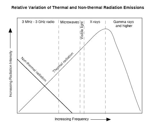
between thermal and non-thermal radiation and give some examples of each. You
will be able to distinguish between thermal and non-thermal radiation curves.
You will be able to describe the significance of the 21-cm hydrogen line in
radio
astronomy.
If the material in this chapter is unfamiliar to you, do not be discouraged if
you don’t understand
everything the first time through. Some of these concepts are a little
complicated and few nonscientists
have much awareness of them. However, having some familiarity with them will
make
your radio astronomy activities much more interesting and meaningful.
What causes electromagnetic radiation to be emitted at different frequencies?
Fortunately for us,
these frequency differences, along with a few other properties we can observe,
give us a lot of
information about the source of the radiation, as well as the media through
which it has traveled.
Electromagnetic radiation is produced by either thermal mechanisms or
non-thermal mechanisms.
Examples of thermal radiation include:
- Continuous spectrum emissions related to the temperature of the object
or
material.
- Specific frequency emissions from neutral hydrogen and other atoms and
molecules.
Examples of non-thermal mechanisms include:
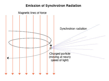
- Emissions due to synchrotron radiation.
- Amplified emissions due to astrophysical masers.
Thermal Radiation -
Back to Table of Contents
Did you know that any object that contains any heat energy at all emits
radiation? When you’re
camping, if you put a large rock in your campfire for a while, then pull it out,
the rock will emit
the energy it has absorbed as radiation, which you can feel as heat if you hold
your hand a few
inches away. Physicists would call the rock a “blackbody” because it absorbs all
the energy that
reaches it, and then emits the energy at all frequencies (although not equally)
at the same rate it
absorbs energy.
All the matter in the known universe behaves this way.
Some astronomical objects emit mostly infrared radiation, others mostly visible
light, others
mostly ultraviolet radiation. The single most important property of objects that
determines the
radiation they emit is temperature.
In solids, the molecules and atoms are vibrating continuously. In a gas, the
molecules are really
zooming around, continuously bumping into each other. Whatever the amount of
molecular
motion occurring in matter, the speed is related to the temperature. The hotter
the material, the
faster its molecules are vibrating or moving.
Electromagnetic radiation is produced whenever electric charges accelerate—that
is, when they
change either the speed or direction of their movement. In a hot object, the
molecules are continuously
vibrating (if a solid) or bumping into each other (if a liquid or gas), sending
each other
off in different directions and at different speeds. Each of these collisions
produces electromagnetic
radiation at frequencies all across the electromagnetic spectrum. However, the
amount of
radiation emitted at each frequency (or frequency band) depends on the
temperature of the
material producing the radiation.
It turns out that the shorter the wavelength (and higher the frequency), the
more energy the
radiation carries. When you are out in the sun on a hot day and your skin starts
to feel hot, that
heat is not what you need to worry about if you get sunburned easily. Most of
the heat you feel is
the result of infrared radiation striking the surface of your skin. However, it
is the higher frequency—
thus higher energy—ultraviolet radiation penetrating the skin’s surface that
stimulates
the deeper layers to produce the melanin that gives fair complected folks the
nice tan—or bad
sunburn. X-rays, at still higher frequencies, have enough energy to pass right
through skin and
other soft tissues. That is how bone and soft tissues of varying densities can
be revealed by the xray
imaging techniques used by medicine.|
Any matter that is heated above absolute zero generates electromagnetic energy.
The intensity of
the emission and the distribution of frequencies on the electromagnetic spectrum
depend upon the
temperature of the emitting matter. In theory, it is possible to detect
electromagnetic energy from
any object in the universe. Visible stars radiate a great deal of
electromagnetic energy. Much of
that energy has to be in the visible part of the spectrum—otherwise they would
not be visible
stars! Part of the energy has to be in the microwave (short wave radio) part of
the spectrum, and
that is the part astronomers study using radio telescopes.
Blackbody Characteristics -
Back to Table of Contents
Blackbodies thus have three characteristics:
- A blackbody with a temperature higher than absolute zero emits some
energy at
all wavelengths.
- A blackbody at higher temperature emits more energy at all wavelengths
than
does a cooler one.
- The higher the temperature, the shorter the wavelength at which the
maximum
energy is emitted.
To illustrate, at a low temperature setting, a burner on an electric stove emits
infrared radiation,
which is transferred to other objects (such as pots and food) as heat. At a
higher temperature, it
also emits red light (lower frequency end of visible light range). If the
electrical circuit could
deliver enough energy, as the temperature increased further, the burner would
turn yellow, or
even blue-white.
The sun and other stars may, for most purposes, be considered blackbodies. So we
can estimate
temperatures of these objects based on the frequencies of radiation they emit—in
other words,
according to their electromagnetic spectra.
For radiation produced by thermal mechanisms, the following table gives samples
of wavelength
ranges, the temperatures of the matter emitting in that range, and some example
sources of such
thermal radiation.
The hotter the object, the shorter is the wavelength of the radiation it
emits. Actually, at hotter
temperatures, more energy is emitted at all wavelengths. But the peak amount of
energy is
radiated at shorter wavelengths for higher temperatures. This relationship is
known as Wien’s
Law.
A beam of electromagnetic radiation can be regarded as a stream of tiny packets
of energy called
photons. Planck’s Law states that the energy carried by a photon is directly
proportional to its
frequency. To arrive at the exact energy value, the frequency is multiplied by
Planck’s Constant,
which has been found experimentally to be 6.625 x 10⁻²⁷ erg sec. (The erg is a
unit of energy.)
If we sum up the contributions from all parts of the electromagnetic spectrum,
we obtain the total
energy emitted by a blackbody over all wavelengths. That total energy, emitted
per second per
square meter by a blackbody at a given temperature is proportional to the fourth
power of its
absolute temperature. This relationship is known as the Stefan-Boltzmann Law. If
the sun, for
example, were twice as hot as it is and the same size, that is, if its
temperature were 11,600 K, it
would radiate 24, or 16, times more energy than it does now.
The flux density of the radiation is defined as the energy received per unit
area per unit of frequency
bandwidth. Astronomers also consider the radiation’s brightness, which is a more
mathematically precise calculation of the energy received per unit area, for a
particular frequency
bandwidth, and also taking into consideration the angle of incidence on the
measuring surface and
the solid angle of sky subtended by the source. The brightness of radiation
received (at all
frequencies) is thus related to temperature of the emitting object and the
wavelength of the
received radiation.
The variation of brightness with frequency is called the brightness spectrum.
The spectral power
is the energy observed per unit of time for a specific frequency bandwidth.
A plot of a brightness spectrum shows the brightness of the radiation received
from a source as it
varies by frequency and wavelength. In the plot below, the brightness of
blackbodies at various
temperatures is plotted on the vertical scale and wavelengths are plotted on the
horizontal scale.
The main thing to notice about these plots is that the curves never cross
each other. Therefore, at
any frequency, there is only one temperature for each brightness. So, if you can
measure the
brightness of the energy at a given frequency, you know the temperature of the
emitting object!
Despite their temperatures, not all visible stars are good radio frequency
emitters. We can detect
stars at radio frequencies only
if they emit by non-thermal
mechanisms (described next), or
if they are in our solar
system (that is, our sun), or
if there is gas beyond the
star which is emitting (for example, a stellar wind).
As it turns out, the hottest and brightest stars emit more energy at
frequencies above the visible
range than below it. Such stars are known for their x-ray and atomic particle
radiation. However,
intense thermal generators such as our own sun emit enough energy in the radio
frequencies to
make them good candidates for radio astronomy studies. The Milky Way galaxy
emits both
thermal and non-thermal radio energy, giving radio astronomers a rich variety of
data to ponder.
Our observations of radiation of thermal origin have two characteristics that
help distinguish it
from other types of radiation. Thermal radiation reproduces on a loudspeaker as
pure static hiss,
and the energy of radiation of thermal origin usually increases with frequency.
Continuum Emissions from Ionized Gas
Thermal blackbody radiation is also emitted by gases. Plasmas are ionized gases
and are considered
to be a fourth state of matter, after the solid, liquid, and gaseous states. As
a matter of fact,
plasmas are the most common form of matter in the known universe (constituting
up to 99% of
it!) since they occur inside stars and in the interstellar gas. However,
naturally occurring plasmas
are relatively rare on Earth primarily because temperatures are seldom high
enough to produce
the necessary degree of ionization. The flash of a lightning bolt and the glow
of the aurora
borealis are examples of plasmas. But immediately beyond Earth’s atmosphere is
the plasma
comprising the Van Allen radiation belts and the solar wind.
An atom in a gas becomes ionized when another atom bombards it with sufficient
energy to
knock out an electron, thus leaving a positively charged ion and a negatively
charged electron.
Once separated, the charged particles tend to recombine with their opposites at
a rate dependent
on the density of the electrons. As the electron and ion accelerate toward one
another, the electron
emits electromagnetic energy. Again, the kinetic energy of the colliding atoms
tends to
separate them into electron and positive ion, making the process continue
indefinitely. The gas
will always have some proportion of neutral to ionized atoms.
As the charged particles move around, they can generate local concentrations of
positive or
negative charge, which gives rise to electric and magnetic fields. These fields
affect the motion
of other charged particles far away. Thus, elements of the ionized gas exert a
force on one
another even at large distances. An ionized gas becomes a plasma when enough of
the atoms are
ionized so that the gas exhibits collective behavior.
Whenever a vast quantity of free and oppositely charged ions coexist in a
relatively small space,
the combination of their reactions can add up to intense, continuous, wideband
radio frequency
radiation. Such conditions prevail around stars, nebulae, clusters of stars, and
even planets—
Jupiter being at least one we know of.
Spectral Line Emissions from Atoms and Molecules
- Back to Table of Contents
While the mechanism behind thermal-related energy emissions from ionized gases
involves
electrons becoming detached from atoms, line emissions from neutral hydrogen and
other atoms
and molecules involves the electrons changing energy states within the atom,
emitting a photon of
energy at a wavelength characteristic of that atom. Thus, this radiation
mechanism is called line
emission, since the wavelength of each atom occupies a discrete “line” on the
electromagnetic
spectrum.
In the case of neutral (not ionized) hydrogen atoms, in their lower energy
(ground) state, the
proton and the electron spin in opposite directions. If the hydrogen atom
acquires a slight amount
of energy by colliding with another atom or electron, the spins of the proton
and electron in the
hydrogen atom can align, leaving the atom in a slightly excited state. If the
atom then loses that
amount of energy, it returns to its ground state. The amount of energy lost is
that associated with
a photon of 21.11 cm wavelength (frequency 1428 MHz).
Hydrogen is the key element in the universe. Since it is the main constituent
of interstellar gas,
we often characterize a region of interstellar space as to whether its hydrogen
is neutral, in which
case we call it an H I region, or ionized, in which case we call it an H II
region.
Some researchers involved in the search for extra-terrestrial intelligence (see
Chapter 8) have
reasoned that another intelligent species might use this universal 21-cm
wavelength line emission
by neutral hydrogen to encode a message; thus these searchers have tuned their
antennas specifically
to detect modulations to this wavelength. But, perhaps more usefully,
observations of this
wavelength have given us much information about the interstellar medium and
locations and
extent of cold interstellar gas.
Non-thermal Mechanisms -
Back to Table of Contents
Radiation is also produced by mechanisms unrelated to the temperature of object
(that is, thermal
radiation). Here we discuss some examples of non-thermal radiation.
Synchrotron Radiation
Notwithstanding the vast number of sources of thermal emissions, much of the
radiation from our
own galaxy, particularly the background radiation first discovered by Jansky,
and most of that
from other galaxies is of non-thermal origin. The major mechanism behind this
type of radiation
has nothing to do with temperature, but rather with the effect of charged
particles interacting with
magnetic fields. When a charged particle enters a magnetic field, the field
compels it to move in a
circular or spiral path around the magnetic lines of force. The particle is thus
accelerated and
radiates energy. Under non-relativistic conditions (that is, when particle
velocities are well-below
the speed of light), this cyclotron radiation is not strong enough to have much
astronomical
importance. However, when the speed of the particle reaches nearly the speed of
light, it emits a
much stronger form of cyclotron radiation called synchrotron radiation.
Quasars (described in Chapter 6) are one source of synchrotron radiation not
only at radio wavelengths,
but also at visible and x-ray wavelengths.
An important difference in radiation from thermal versus non-thermal mechanisms
is that while
the intensity (energy) of thermal radiation increases with frequency, the
intensity of non-thermal
radiation usually decreases with frequency.
Masers - Back to Table
of Contents
Astronomical masers are another source of non-thermal radiation. “Maser” is
short for microwave-
amplified stimulated emission of radiation. Masers are very compact sites within
molecular
clouds where emission from certain molecular lines can be enormously amplified.
The interstellar
medium contains only a smattering of molecular species such as water (H2O),
hydroxl radicals
(OH), silicon monoxide (SiO), and methanol (CH3OH). Normally, because of the
scarcity of
these molecules, their line emissions would be very difficult to detect with
anything but very
crude resolution. However, because of the phenomenon of “masing,” these clouds
can be
detected in other galaxies!
In simplified terms, masing occurs when clouds of these molecules encounter an
intense radiation
field, such as that from a nearby source such as a luminous star, or when they
collide with the far
more abundant H2 molecules. What is called a “population inversion” occurs, in
which there are
more molecules in an excited state (that is, their electrons have “jumped” to a
higher energy
level), than in a stable, ground state. This phenomenon is called pumping. As
the radiation
causing the pumping travels through the cloud, the original ray is amplified
exponentially,
emerging at the same frequency and phase as the original ray, but greatly
amplified. Some
masers emit as powerfully as stars! This phenomenon is related to that of
spectral line emissions,
explained in Chapter 4.
Incidentally, this same principle is used in a device called a maser amplifier,
which is installed as
part of some radio telescopes (not in the GAVRT, however) to amplify the signal
received by the
antenna.
Back to Top |
Back to
Astronomy Tools
Chapter 4 -
Back to Table of Contents
Effects of Media
Objectives: When you have completed this chapter, you will be able to describe
several
important variables in the media through which the radiation passes and how they
affect the particles/waves arriving at the telescope. You will be able to
describe
atmospheric “windows” and give an example. You will be able to describe the
effects of absorbing and dispersing media on wave propagation. You will be able
to describe Kirchhoff’s laws of spectral analysis, and give examples of sources
of
spectral lines. You will be able to define reflection, refraction,
superposition,
phase, interference, diffraction, scintillation, and Faraday rotation.
Electromagnetic radiation from space comes in all the wavelengths of the
spectrum, from gamma
rays to radio waves. However, the radiation that actually reaches us is greatly
affected by the
media through which it has passed. The atoms and molecules of the medium may
absorb some
wavelengths, scatter (reflect) other wavelengths, and let some pass through only
slightly bent
(refracted).
Atmospheric “Windows” -
Back to Table of Contents
Earth’s atmosphere presents an opaque barrier to much of the electromagnetic
spectrum. The
atmosphere absorbs most of the wavelengths shorter than ultraviolet, most of the
wavelengths
between infrared and microwaves, and most of the longest radio waves. That
leaves only visible
light, some ultraviolet and infrared, and short wave radio to penetrate the
atmosphere and bring
information about the universe to our Earth-bound eyes and instruments.
The main frequency ranges allowed to pass through the atmosphere are referred to
as the radio
window and the optical window. The radio window is the range of frequencies from
about 5
MHz to over 300 GHz (wavelengths of almost 100 m down to about 1 mm). The
low-frequency
end of the window is limited by signal absorption in the ionosphere, while the
upper limit is
determined by signal attenuation caused by water vapor and carbon dioxide in the
atmosphere.
The optical window, and thus optical astronomy, can be severely limited by
atmospheric conditions
such as clouds and air pollution, as well as by interference from artificial
light and the
literally blinding interference from the sun’s light. Radio astronomy is not
hampered by most of
these conditions. For one thing, it can proceed even in broad daylight. However,
at the higher
frequencies in the atmospheric radio window, clouds and rain can cause signal
attenuation. For
this reason, radio telescopes used for studying sub-millimeter wavelengths are
built on the highest
mountains, where the atmosphere has had the least chance for attenuation.
(Conversely, most
radio telescopes are built in low places to alleviate problems with
human-generated interference,
as will be explained in Chapter 6.)
Absorption and Emission Lines -
Back to Table of Contents
As described in Chapter 3, a blackbody object emits radiation of all
wavelengths. However,
when the radiation passes through a gas, some of the electrons in the atoms and
molecules of the
gas absorb some of the energy passing through. The particular wavelengths of
energy absorbed
are unique to the type of atom or molecule. The radiation emerging from the gas
cloud will thus
be missing those specific wavelengths, producing a spectrum with dark absorption
lines.
The atoms or molecules in the gas then re-emit energy at those same wavelengths.
If we can
observe this re-emitted energy with little or no back lighting (for example,
when we look at
clouds of gas in the space between the stars), we will see bright emission lines
against a dark
background. The emission lines are at the exact frequencies of the absorption
lines for a given
gas. These phenomena are known as Kirchhoff’s laws of spectral analysis:
- When a continuous spectrum is viewed through some cool gas, dark
spectral
lines (called absorption lines) appear in the continuous spectrum.
- If the gas is viewed at an angle away from the source of the continuous
spectrum,
a pattern of bright spectral lines (called emission lines) is seen against an
otherwise
dark background.
The same phenomena are at work in the non-visible portions of the spectrum,
including the radio
range. As the radiation passes through a gas, certain wavelengths are absorbed.
Those same
wavelengths appear in emission when the gas is observed at an angle with respect
to the radiation
source.
Why do atoms absorb only electromagnetic energy of a particular wavelength? And
why do they
emit only energy of these same wavelengths? What follows here is a summarized
explanation,
but for a more comprehensive one, see Kaufmann’s Universe, pages 90-96.
The answers lie in quantum mechanics. The electrons in an atom may be in a
number of allowed
energy states. In the atom’s ground state, the electrons are in their lowest
energy states. In order
to jump to one of a limited number of allowed higher energy levels, the atom
must gain a very
specific amount of energy. Conversely, when the electron “falls” to a lower
energy state, it
releases a very specific amount of energy. These discrete packets of energy are
called photons.
Thus, each spectral line corresponds to one particular transition between energy
states of the
atoms of a particular element. An absorption line occurs when an electron jumps
from a lower
energy state to a higher energy state, extracting the required photon from an
outside source of
energy such as the continuous spectrum of a hot, glowing object. An emission
line is formed
when the electron falls back to a lower energy state, releasing a photon.
The diagram on the next page demonstrates absorption and emission of photons by
an atom using
the Neils Bohr model of a hydrogen atom, where the varying energy levels of the
electron are
represented as varying orbits around the nucleus. (We know that this model is
not literally true,
but it is useful for describing electron behavior.) The varying series of
absorption and emission
lines represent different ranges of wavelengths on the continuous spectrum. The
Lyman series,
for example, includes absorption and emission lines in the ultraviolet part of
the spectrum.
Emission and absorption lines are also seen when oppositely charged ions
recombine to an
electrically neutral state. The thus formed neutral atom is highly excited, with
electrons
transitioning between states, emitting and absorbing photons. The resulting
emission and absorption
lines are called recombination lines. Some recombination lines occur at
relatively low
frequencies, well within the radio range, specifically those of carbon ions.
Molecules, as well as atoms, in their gas phase also absorb characteristic
narrow frequency bands
of radiation passed through them. In the microwave and long wavelength infrared
portions of the
spectrum, these lines are due to quantized rotational motion of the molecule.
The precise frequencies
of these absorption lines can be used to determine molecular species. This
method is
valuable for detecting molecules in our atmosphere, in the atmospheres of other
planets, and in
the interstellar medium. Organic molecules (that is, those containing carbon)
have been detected
in space in great abundance using molecular spectroscopy. Molecular spectroscopy
has become
an extremely important area of investigation in radio astronomy.
As will be discussed in Chapter 5, emission and absorption lines in all spectra
of extraterrestrial
origin may be shifted either toward higher (blue) or lower (red) frequencies,
due to a variety of
mechanisms.
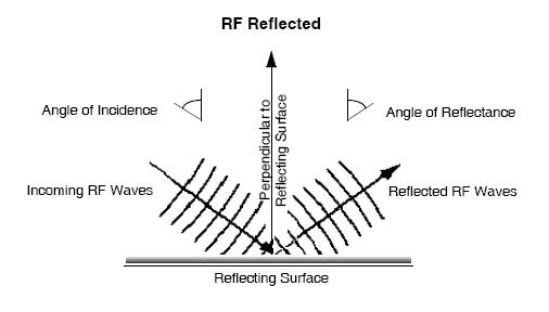
Reflection -
Back to Table of Contents
RF radiation generally travels through space in a straight line. RF waves can be
reflected by
certain substances, much in the same way that light is reflected by a mirror.
The angle at which a
radio wave is reflected from a smooth metal surface, for example, will equal the
angle at which it
approached the surface. In other words, the angle of reflection of RF waves
equals their angle of
incidence.
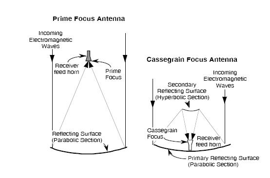
This principle of RF reflection is used in antenna design to focus
transmitted waves into a narrow
beam and to collect and concentrate received RF signals for a receiver. If a
reflector is designed
with the reflecting surface shaped like a paraboloid, electromagnetic waves
approaching parallel
to the axis of the antenna will be reflected and will focus above the surface of
the reflector at the
feed horn. This arrangement is called prime focus and provides the large
aperture (that is,
antenna surface area) necessary to receive very weak signals.
However, a major problem with prime focus arrangements for large aperture
antennas is that the
equipment required at the prime focus is heavy and the supporting structure
tends to sag under the
weight of the equipment, thus affecting calibration. A solution is the
Cassegrain focus arrangement.
Cassegrain antennas add a secondary reflecting surface to “fold” the
electromagnetic
waves back to a prime focus near the primary reflector. The DSN’s antennas
(including the
GAVRT) are of this design because it accommodates large apertures and is
structurally strong,
allowing bulky equipment to be located nearer the structure’s center of gravity.
The reflective properties of electromagnetic waves have also been used to
investigate the planets
using a technique called planetary radar. With this technique, electromagnetic
waves are transmitted
to the planet, where they reflect off the surface of the planet and are received
at one or
more Earth receiving stations. Using very sophisticated signal processing
techniques, the receiving
stations dissect and analyze the signal in terms of time, amplitude, phase, and
frequency.
JPL’s application of this radar technique, called Goldstone Solar System Radar (GSSR),
has been
used to develop detailed images and measurements of several main belt and
near-Earth asteroids.
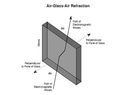
Refraction -
Back to Table of Contents
Refraction is the deflection or bending of electromagnetic waves when they pass
from one kind of
transparent medium into another. The index of refraction is the ratio of the
speed of electromagnetic
energy in a vacuum to the speed of electromagnetic energy in the observed
medium. The
law of refraction states that electromagnetic waves passing from one medium into
another (of a
differing index of refraction) will be bent in their direction of travel.
Usually, substances of higher densities have higher indices of refraction. The
index of refraction
of a vacuum, by definition, is 1.0. The index of refraction of air is 1.00029,
water is 1.3, glass
about 1.5, and diamonds 2.4. Since air and glass have different indices of
refraction, the path of
electromagnetic waves moving from air to glass at an angle will be bent toward
the perpendicular
as they travel into the glass. Likewise, the path will be bent to the same
extent away from the
perpendicular when they exit the other side of glass.
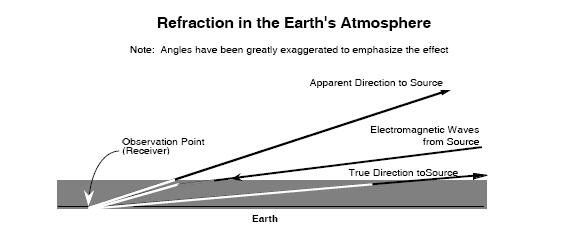
In a similar manner, electromagnetic waves entering Earth's atmosphere from
space are slightly
bent by refraction. Atmospheric refraction is greatest for radiation from
sources near the horizon
(below about 15° elevation) and causes the apparent altitude of the source to be
higher than the
true height. As Earth rotates and the object gains altitude, the refraction
effect decreases, becoming
zero at zenith (directly overhead). Refraction's effect on sunlight adds about 5
minutes to the
daylight at equatorial latitudes, since the sun appears higher in the sky than
it actually is.
Superposition -
Back to Table of Contents
Many types of waves, including electromagnetic waves, have the property that
they can traverse
the same space independently of one another. If this were not the case, we would
be unable to
see anything. Imagine you are standing at one end of a room in an art museum,
trying to view a
painting on the far wall and this property did not apply. The light waves from
all of the paintings
on the side walls crossing back and forth would disrupt the light waves coming
directly to you
from the painting you were trying to view, and the world would be nothing but a
blur. All these
electromagnetic waves do, in fact, additively combine their electric fields at
the point where they
cross. Once they have crossed, each wave resumes in its original direction of
propagation with its
original wave form. This phenomenon is called the property of superposition.
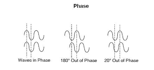
Phase - Back to Table
of Contents
As applied to waves of electromagnetic radiation, phase is the relative measure
of the alignment
of two wave forms of similar frequency. They are said to be in phase if the
peaks and troughs of
the two waves match up with each other in time. They are said to be out of phase
to the extent
that they do not match up. Phase is expressed in degrees from 0 to 360.
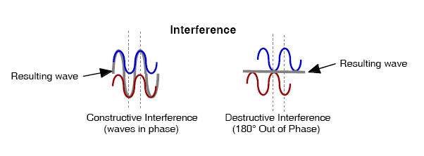
Interference -
Back to Table of Contents
When two waves of the same frequency and moving in the same direction meet, the
resulting
wave is the additive combination of the two waves. In the special case where two
waves have the
same electric field amplitude (wave height) and are in phase, the resulting
amplitude is twice the
original amplitude of each wave and the resulting frequency is the same as the
original frequency
of each wave. This characteristic is called constructive interference. In the
special case where
two waves have the same electric field amplitude and are 180° out of phase, the
two waves cancel
each other out. This characteristic is called destructive interference.
Diffraction -
Back to Table of Contents
When an electromagnetic wave passes by an obstacle in space, the wave is bent
around the object.
This phenomenon is known as diffraction. The effects of diffraction are usually
very small, so we
seldom notice it.
However, you can easily see the effect of diffraction for yourself. All you need
is a source of
light, such as a fluorescent or incandescent light bulb. Hold two fingers about
10 cm in front of
one eye and make the space between your fingers very small, about 1 mm. Now look
through the
space between your fingers at the light source. With a little adjustment of the
spacing, you will
see a series of dark and light lines. These are caused by constructive and
destructive interference
of light diffracting around your fingers.
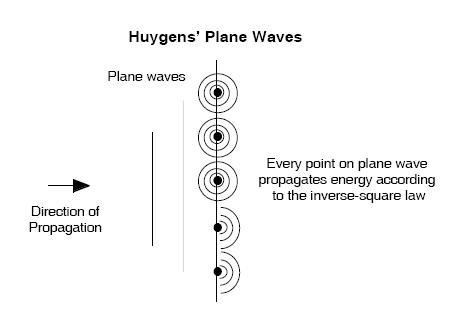
The reason diffraction occurs is not exactly obvious. Christian Huygens in the
mid-1600s offered
an explanation that, strange though it may seem, still nicely explains the
observations. You will
recall the inverse-square law of electromagnetic propagation from Chapter 2.
Electromagnetic
energy may be considered to propagate from a point source in plane waves. (The
illustration of
reflection on page 34 shows the RF waves as planes.) The inverse square law
applies not only to
the source of the energy but also to any point on a plane wave. That is, from
any point on the
plane wave, the energy is propagated as if the point were the source of the
energy. Thus, waves
may be considered to be continuously created from every point on the plane and
propagated in
every direction.
For an infinite plane wave, the sideways propagation from each point is
balanced by the propagation
from its neighbors, so the wave continues on as a plane. However, when a wave
encounters
an object, the effect at the edges of the object is that the path of the
radiation is slightly bent.
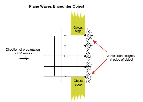
Now suppose the radiation (for example, light) is then intercepted by a
surface (such as a screen)
a short distance from the object. Then, compared to the parallel waves that have
passed farther
from the object’s edge (for example “waves B, C, and D” in the illustration
below), the waves
that have bent around the edges of the object (“waves A and E” for example) will
have travelled a
shorter or longer distance from the object to any given point on the screen.
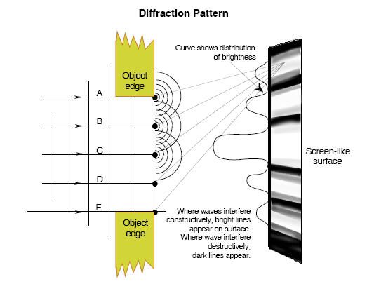
The effect is that the light waves are out of phase when they arrive at any
given point on the
surface. If they are 180° out of phase, they cancel each other out (destructive
interference) and
produce a dark line. If they are in phase, they add together (constructive
interference) and
produce a bright line.
Diffraction is most noticeable when an electromagnetic wave passing around an
obstacle or
through an opening in an obstacle (such as the slit between your fingers) is all
of the same
frequency, or monochromatic.
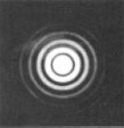
The picture below shows a typical diffraction pattern seen when observing a star
through a
telescope with a lens that focuses the light to a point (a converging lens).
Scintillation -
Back to Table of Contents
As electromagnetic waves travel through Earth’s atmosphere, they pass through
areas of varying
pressure, temperature, and water content. This dynamic medium has rapidly
varying indices of
refraction, causing the waves to take different paths through the atmosphere.
The consequence is
that at the point of observation, the waves will be out of phase and appear to
be varying in
intensity. The effect in the visual range is that stars appear to twinkle and
distant scenes on the
horizon appear to shimmer (for example, when we see distant “water” mirages in
the hot desert).
In the radio range, the same phenomenon is called scintillation. The
interplanetary and interstellar
media can have a similar effect on the electromagnetic waves passing through
them.
A star will scintillate or twinkle most violently when it is low over the
horizon, as its radiation
passes through a thick layer of atmosphere. A planet, which appears as a small
disk, rather than a
point, will usually scintillate much less than a star, because light waves from
one side of the disk
are “averaged” with light waves coming from other parts of the disk to smooth
out the overall
image.
Technology has been developed for both radio and optical telescopes to
significantly cancel out
the phase changes observed for a given source, thus correcting the resulting
distortion. This
technology is not implemented on the GAVRT.
Faraday Rotation -
Back to Table of Contents
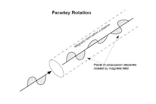
Faraday rotation (or Faraday effect) is a rotating of the plane of polarization
of the linearly
polarized electromagnetic waves as they pass through a magnetic field in a
plasma. A linearly
polarized wave may be thought of as the sum of two circularly polarized waves of
opposite hand.
That is, one wave is polarized to the right and one wave is polarized to the
left. (Both waves are
at the same frequency.) When the linearly polarized wave passes through a
magnetic field, the
right polarized wave component travels very slightly faster than the left
polarized wave component.
Over a distance, this phenomenon has the effect of rotating the plane of the
linearly polarized
wave. A measure of the amount of rotation can give a value of the density of a
plasma.
Back to Top |
Back to
Astronomy Tools
Chapter 5 -
Back to Table of Contents
Effects of Motion and Gravity
Objectives: When you have completed this chapter, you will be able to describe
the Doppler
effect on the frequency of the received particles/waves; describe the
significance
of spectral red shifting and blue shifting; describe the effects of gravity on
electromagnetic radiation; describe superluminal expansion; and define
occultation.
Doppler Effect -
Back to Table of Contents
Regardless of the frequency of electromagnetic waves, they are subject to the
Doppler effect.
The Doppler effect causes the observed frequency of radiation from a source to
differ from the
actual radiated frequency if there is motion that is increasing or decreasing
the distance between
the source and the observer. The same effect is readily observable as variation
in the pitch of
sound between a moving source and a stationary observer, or vice versa.
When the distance between the source and receiver of electromagnetic waves
remains constant,
the frequency of the source and received wave forms is the same. When the
distance between the
source and receiver of electromagnetic waves is increasing, the frequency of the
received wave
forms is lower than the frequency of the source wave form. When the distance is
decreasing, the
frequency of the received wave form will be higher than the source wave form.
The Doppler effect is very important to both optical and radio astronomy. The
observed spectra
of objects moving through space toward Earth are shifted toward the blue
(shorter wavelengths),
while objects moving through space away from Earth are shifted toward the red.
The Doppler
effect works at all wavelengths of the electromagnetic spectrum. Thus, the
phenomenon of
apparent shortening of wavelengths in any part of the spectrum from a source
that is moving
toward the observer is called blue shifting, while the apparent lengthening of
wavelengths in any
part of the spectrum from a source that is moving away from the observer is
called red shifting.
Relatively few extraterrestrial objects have been observed to be blue shifted,
and these, it turns
out, are very close by, cosmically speaking. Examples are planets in our own
solar system with
which we are closing ranks due to our relative positions in our orbits about the
sun, some other
objects in our galaxy, some molecular clouds, as well as some galaxies in what
is termed the
local group of galaxies.
Almost all other distant objects are red shifted. The red shifting of spectra
from very distant
objects is due to the simple fact that the universe is expanding. Space itself
is expanding between
us and distant objects, thus they are moving away from us. This effect is called
cosmic red
shifting, but it is still due to the Doppler effect.
Distances to extragalactic objects can be estimated based in part on the degree
of red shifting of
their spectra. As the universe expands, all objects recede from one another at a
rate proportional
to their distances. The Hubble Constant relates the expansion velocity to the
distance and is most
important for estimating distances based on the amount of red shifting of
radiation from a source.
Our current estimate for the Hubble Constant is 60-80 km/s per million parsecs (1
parsec = 3.26
light years).
The spectra from quasars, for example, are quite red-shifted. Along with other
characteristics,
such as their remarkable energy, this red shifting suggests that quasars are the
oldest and most
distant objects we have observed. The most distant quasars appear to be receding
at over 90% the
speed of light!
Gravitational Red Shifting -
Back to Table of Contents
Red shifting, of course, indicates an elongating of the wavelength. An elongated
wavelength
indicates that the radiation has lost some of its energy from the instant it
left its source.
As predicted by Einstein, radiation also experiences a slight amount of red
shifting due to gravitational
influences. Gravitational red shifting is due to the change in the strength of
gravity and
occurs mostly near massive bodies. For example, as radiation leaves a star, the
gravitational
attraction near the star produces a very slight lengthening of the wavelengths,
as the radiation
loses energy in its effort to escape the pull of gravity from the large mass.
This red shifting
diminishes in effect as the radiation travels outside the sphere of influence of
the source’s gravity.
Gravitational Lensing -
Back to Table of Contents
Einstein’s theory of general relativity predicts that space is actually warped
around massive
objects.
In 1979, astronomers noticed two remarkably similar quasars very close together.
They had the
same magnitude, spectra, and red shift. They wondered if the two images could
actually represent
the same object. It turned out that a galaxy lay directly in the path between
the two quasars
and Earth, much closer to Earth than the quasars. The geometry and estimated
mass of the
galaxy were such that it produced a gravitational lens effect—that is, a warping
of the light as it
passes through the space around the galaxy.
Many other instances of gravitational lensing have now been detected.
Gravitational lensing can
produce more than two images, or even arcs. Images produced by point-like
gravitational lenses
can appear much brighter than the original source would appear in the absence of
the gravitational
lens.
Superluminal Velocities -
Back to Table of Contents
Some discrete (defined in the next chapter) sources within quasars have been
observed to change
positions over a brief period. Their motion generally appears to the observer to
be radially
outward from the center of the quasar image. The apparent velocities of these
objects have been
measured, and if the red shifts actually do represent the distance and recession
velocities of the
quasar, then these discrete objects are moving at speeds greater than the speed
of light! We call
these apparent speeds superluminal velocities or superluminal expansion.
Well, we know this is impossible, right? So astronomers had to come up with a
more reasonable
explanation. The most widely accepted explanation is that the radiation emitted
from the object
at the first position (A in the diagram below) has traveled farther and thus
taken longer to reach
Earth than the radiation emitted from the second position (B), 5 LY from A.
Suppose A is 4 light years (LY) farther from Earth than B (that is, AC is 4
LY). Moving just a bit
under the speed of light, the object takes just over 5 LY to travel from A to B.
However, the
radiation it emitted at A reaches C in 4 years. As that radiation continues
toward Earth, it is one
year ahead of the radiation emitted toward us by the object when it arrived at
B. When it finally
(after several billion years) reaches Earth, the radiation from A is still one
year ahead of the
radiation from B. It appears to us that the object has moved tangentially out
from the center of
the quasar, from C to B and (from the Pythagorean theorem) has gone 3 LY in just
over one year!
That the object appears to travel at nearly three times light speed is only
because of the projection
effect, with its radiation traveling from A to C in 4 years, while the object
itself went from A to
B in 5 years.
Occultations -
Back to Table of Contents
When one celestial body passes between Earth and another celestial body, we say
that the object
that is wholly or partially hidden from our view is occulted. Examples of
occultations are the
moon passing in front of a star or a planet, or a planet passing in front of a
star, or one planet
passing in front of another planet, such as in 1590 when Venus occulted Mars.
An occultation can provide an unparalleled opportunity to study any existing
atmosphere on the
occulting planet. As the radiation from the farther object passes through the
atmosphere at the
limb of the nearer object, that radiation will be influenced according to the
properties of that
atmosphere. The degree of refraction of the radiation gives information about
the atmosphere’s
density and thickness. Spectroscopic studies give information about the
atmosphere’s composition.
Back to Top |
Back to
Astronomy Tools
Chapter 6 -
Back to Table of Contents
Sources of Radio Frequency Emissions
Objectives: Upon completion of this chapter, you will be able to define and give
examples of
a “point source,” a “localized source,” and an “extended source” of radio
frequency
emissions; distinguish between “foreground” and “background” radiation;
describe the theoretical source of “cosmic background radiation”; describe a
radio star, a flare star, and a pulsar; explain why pulsars are sometimes
referred
to as standard clocks; describe the relationship between pulsar spin down and
age; describe “normal” galaxies and “radio” galaxies; describe the general
characteristics of the emissions from Jupiter, Io, and the Io plasma torus;
describe
the impact of interference on radio astronomy observations; and describe a major
source of natural interference and of human made interference.
Classifying the Source -
Back to Table of Contents
Radiation whose direction can be identified is said to originate from a discrete
source. A discrete
source often can be associated with a visible (whether by the naked eye or by
optical
telescope) object. For example, a single star or small group of stars viewed
from Earth is a
discrete source. Our sun is a discrete source. A quasar is a discrete source.
However, the
definition of “discrete,” in addition to the other terms used to describe the
extent of a source,
often depends upon the beam size of the radio telescope antenna being used in
the observation.
Discrete sources may be further classified as point sources, localized sources,
and extended
sources.
A point source is an idealization. It is defined as a source that subtends an
infinitesimally small
angle. All objects in reality subtend at least a very tiny angle, but often it
is mathematically
convenient for astronomers to regard sources of very small extent as point
sources. Objects that
appear smaller than the telescope’s beam size are often called “unresolved”
objects and can
effectively be treated as point sources. A localized source is a discrete source
of very small
extent. A single star may be considered a localized source.
Emitters of radiation that covers a relatively large part of the sky are called
extended sources.
An example of an extended source of radiation is our Milky Way galaxy, or its
galactic center
(called Sagittarius A) from which radiation emissions are most intense.

An optical analogy to the extended source would be the view of a large city
at night from an
airplane at about 10 km altitude. All the city lights would tend to blend
together into an apparently
single, extended source of light. On the other hand, a single searchlight viewed
from the
same altitude would stand out as a single object, analogous to a localized or
point source.
The terms localized and extended are relative and depend on the precision with
which the telescope
observing them can determine the source.
Background radiation is radio frequency radiation that originates from farther
away than the
object being studied, whereas foreground radiation originates from closer than
the object being
studied. If an astronomer is studying a specific nearby star, the radiation from
the Milky Way
may be considered not merely an extended source, but background radiation. Or,
if it is a distant
galaxy being observed, the Milky Way may be considered a pesky source of
foreground radiation.
Background and foreground radiation may consist of the combined emissions from
many discrete
sources or may be a more or less continuous distribution of radiation from our
galaxy.
Cosmic background radiation, on the other hand, is predicted to remain as the
dying glow from
the big bang. It was first observed by Arno Penzias and Robert Wilson in 1965.
(They won a
Nobel Prize for this discovery in 1978). As discussed in Chapter 3, much of
background and
foreground radiation tends to be of non-thermal origin. The cosmic background
radiation,
however, is thermal.
In the group of pictures below (from Griffith Observatory and JPL), the entire
sky is shown at (a)
radio, (b) infrared, (c) visible, and (d) X-ray wavelengths. Each illustration
shows the Milky Way
stretching horizontally across the picture. It is clear that radio wavelengths
give us a very different
picture of our sky.
Star Sources -
Back to Table of Contents
Many thousands of visible stellar objects have been discovered to also be strong
emitters of radio
frequency radiation. All such stars may be called radio stars.
It is helpful in discussing star types and activities to review stellar
evolution. For a discussion of
star birth, maturation, old age, and death, please read Chapters 20-22 in
Universe, by William J.
Kaufmann III, or Chapters 28-30 in Abell’s Exploration of the Universe, by David
Morrison,
Sidney Wolff, and Andrew Fraknoi.
Variable Stars -
Back to Table of Contents
Stars do not shine uniformly brightly all the time. Stars that show significant
changes in brightness
over periods we short-lived humans can perceive are of great importance to
astronomy
because of what we can surmise from those changes. And fortunately for radio
astronomy, it has
been discovered that stars whose output of visible radiation varies over short
periods, either
regularly or irregularly, have corresponding variations in their output of radio
frequency emissions.
Some variable stars , such as Cepheids (SEE-fee-ids), are absolutely regular
in their cyclic
changes, varying from a few days to a few weeks. It has been found that stars
with longer regular
periods are always more luminous (emitting more energy) than those with shorter
regular periods.
Variable stars with very short periods (1.25 to 30 hours) are called RR Lyrae
variables. None of
these shorter period variables is bright enough to see with the naked eye.
Because the intrinsic
luminosities of Cepheids and RR Lyraes with similar periods are comparable,
variable stars such
as these can be used to work out interstellar and even intergalactic distances.
Other variable stars have much longer periods, are less regular in their cycles,
and vary by a much
greater magnitude. These are called semi-regular variables. The red giant
Betelgeuse in the
Orion constellation is an example. No period-luminosity relationship has been
found for semiregular
variables.
Irregular variables have no set periods at all. They usually are young stars and
their luminosities
may vary over a very large range.
Flare stars are faint red dwarf stars (older and feebler than white dwarfs) that
exhibit sudden
increases in brightness over a period of a few minutes due to intense flare
activity, fading back to
their usual brightness within an hour or so. Typical flare stars are UV Ceti and
AD Leonis.
Binary (double) stars may produce apparently regularly varying radiation if the
two stars eclipse
one another in their orbits. Also, radio emissions from binaries are more common
than for single
stars. The interaction of stellar winds and magnetospheres, bow shocks, and
tidal effects may
contribute to the conditions producing radio frequency emissions.
Pulsars - Back to Table
of Contents
Sometimes when a star goes supernova, all that is left after this most violent
of processes is a
cloud of expanding gas and the tiny remnant of extremely dense material only a
few tens of
kilometers in diameter. The supernova implosion is so intense that the protons
and electrons in
the atoms of the star are jammed together, thus canceling out their electrical
charges and forming
neutrons. This neutron star may be 1014 times as dense as water! It will have
extremely powerful
magnetic fields and may rotate very rapidly. Because the magnetic axis may not
correspond
to the spin axis, a beam of radiation emitted from the magnetic poles may seem
to an observer to
pulse like a rotating searchlight. Thus we call these rotating neutron stars
pulsars. Although
some pulsars are seen at visible and x-ray frequencies, many more are seen at
radio frequencies.
Since 1967, when the first pulsar was detected by Jocelyn Bell, hundreds of
pulsars have been
discovered. The Crab pulsar spins at 30 times per second. The pulsar 1937+21 in
Cygnus pulses
642 times per second. We receive this emission on Earth as if it were a signal
produced by a
cosmic clock. Over the brief period we have been observing them, however, they
all them seem
to be gradually slowing down. Their energy is dissipating with age. After
correction for this
effect, some millisecond pulsars are at least as accurate at timekeeping as the
best atomic clocks.
The rate at which pulsars slow down has been helpful in confirming aspects of
Einstein’s theory
of general relativity. Also, the timing of pulsars can be useful in determining
properties of the
interstellar medium.
Our Sun -
Back to Table of Contents
The strongest extraterrestrial radio source we experience here on Earth is our
own star. The Sun
is a very ordinary star—not particularly massive or small, not particularly hot
or cold, not particularly
young or old. Perhaps we are fortunate it is so typical because from it we can
learn much
about stars in general.
The photosphere is the part of the sun’s atmosphere that emits most of the
visible light, while the
corona, the sun’s outer atmosphere, is much less dense and emits only a very
small amount of
visible light. The chromosphere, cool and dim compared to the photosphere, forms
the boundary
between the photosphere and the corona.
The sun seems to have about an 11-year cycle of activity. When the sun is in a
quiet phase, radio
emissions from the photosphere (the part that also emits radiation in the
visible wavelength) are
in the wavelength range of 1 cm, while radio emissions from the corona approach
a wavelength
of one meter. The size of the radio solar disk appears only slightly larger than
the optical solar
disk as long as the telescope is tuned to only the 1-cm to 10-cm wavelength
range. But at the
longer wavelengths, the radio solar disk is much larger, including, as it does,
the corona, which
extends millions of kilometers above the photosphere.
Sunspots are darker appearing areas on the photosphere, and, as mentioned above,
they seem to
fluctuate in frequency over about an 11-year cycle. They appear darker because
they are a “cool”
4,000°C relative to the surrounding 6,000°C surface. They are the centers of
magnetic fields,
apparently related to the sun’s magnetic field. It is possible that the sun’s
magnetic lines of force
periodically get “tangled” and destabilized since the sun’s rate of rotation
varies from the equator
to the poles. Solar flares breaking out of the sun’s upper atmosphere are
usually associated with
sunspot groups.
Solar flares emit short bursts of radio energy, with wavelengths observable
from the ground from
about 1 to 60 m (300-5 MHz). Sometimes during intense flares, a stream of
high-energy cosmic
ray particles is emitted, traveling at over 500-1000 km per sec. When these
charged particles
reach Earth’s magnetic field, we get magnetic storms and the aurora. The pattern
of radio emissions
from solar flares appears to originate from a larger area of the solar surface
than does the
pattern of visible-range radiation, but it is still apparent that they are the
result of the same
activity.
The radiation associated with solar flares is circularly polarized, rather than
randomly polarized
as is usual from extraterrestrial sources. This polarization may be caused by
electrons gyrating in
the localized, intense magnetic field of the flare.
The sun is studied by radio astronomers both directly, by observing the actual
radio emissions
from the sun, and indirectly, by observing the effect of the sun’s radiation on
Earth’s ionosphere.
Galactic and Extragalactic Sources
- Back to Table of Contents
We can think of extra-terrestrial radio emissions as originating either within
our galaxy or outside
our galaxy. Inside our galaxy, remnants of supernova explosions are strong
sources of radio
emissions.
Outside our galaxy, we find great variation in the radio emissions from
different galaxies. So we
have arbitrarily divided these other galaxies into “normal” and “active”
galaxies.
Normal galaxies are not very strong sources. For example, the Great Andromeda
Spiral, the
largest galaxy in our so-called local group of galaxies, emits 1032 watts of
power. In contrast,
Cygnus A, over half a billion light years from Earth, is one of the most
conspicuous radio sources
in the sky, with a power output of 1038 watts. (See figures at end of Chapter 8
for a rough idea of
the locations of these galaxies.)
Active galaxies include radio galaxies, quasars, blasars, and Seyfert Galaxies.
Radio galaxies emit a very large quantity of radio waves.
Quasars, coined from the phrase “quasi-stellar radio source,” may be pouring out
energy a
million times more powerfully than a normal galaxy. Quasars are the most distant
objects we
have detected, some approaching 15 billion light years distant—their radiation
requiring nearly
the age of the universe to reach us. And some seem to be receding from us at a
rate 90% the
speed of light.
Blasars are galaxies with extremely bright centers, whose luminosity seems to
vary markedly
over a very short period.
Seyfert galaxies are also intense sources of radiation whose spectra include
emission lines.
In all these, the predominant radiation-producing mechanism is synchrotron
radiation. An active
galaxy may radiate 1,000,000 times more powerfully in the radio frequencies than
a normal
galaxy. Much of the radiation often seems to come from the nucleus of the
galaxy. Astronomers
are now investigating the plausibility of a “unified theory of active galaxies,”
which would
account for the varying behavior observed by all these types of active galaxies.
It may be that
these galaxies have a black hole or a supermassive black hole at their centers,
and their appearance
to us depends on the angle at which we are observing them.
Please read Chapter 27 of
Universe, by Kaufmann, for more information,
including many color
photos, about these fascinating and mysterious objects.
Planetary Sources and Their Satellites -
Back to Table of Contents
Unlike stars, the radio energy observed from planets and their satellites
(except the Jupiter system
and, to a small extent, Saturn) is mostly thermal blackbody radiation. The
wavelengths of
radiation observed from these bodies gives us fairly precise indications of
their temperatures, both
at their surfaces and at varying depths beneath their surfaces.
The Jupiter System -
Back to Table of Contents
By far the most interesting planet for radio astronomy studies is
Jupiter. As
beautiful and fascinating
as it is visually, it is even more fascinating and complex to observe in the
radio frequency
range. Most of the radiation from the Jupiter system is much stronger at longer
wavelengths than
would be expected for thermal radiation. In addition, much of it is circularly
or elliptically
polarized—not at all typical of thermal radiation. Thus, it must be concluded
that non-thermal
processes similar to those taking place in galaxies are at work. That is, ions
and electrons accelerated
by the planet’s spinning magnetic field are generating synchrotron radiation.
Jupiter is 318 times as massive as Earth. Its magnetic axis is tilted 15° from
its rotational axis
and offset from the planet’s center by 18,000 km. Its polarity is opposite that
of Earth (that is, a
compass needle would point south).
Jupiter’s surface magnetic field is 20 to 30 times as strong as that of Earth.
The magnetosphere
of a planet is the region around it in which the planet’s magnetic field
dominates the interplanetary
field carried by the solar wind. If we could see Jupiter’s magnetosphere from
Earth, it
would appear as large as our moon!
The farther a planet is from the sun, the weaker will be the pressure from the
solar wind on the
planet’s magnetosphere. Thus, Jupiter’s magnetic field, already quite intense,
has considerably
less pressure holding it close to the planet than does Earth’s magnetic field.
Jupiter’s magnetosphere
expands and contracts with variations in the solar wind. Its upstream (closest
to the sun)
boundary (called the bowshock) varies from 50 to 100 Jupiter radii and envelopes
Jupiter’s four
large Galilean satellites. (Sixteen Jupiter satellites have been discovered; the
Galilean satellites
are by far the largest).
The magnetosphere of a planet traps plasma, as magnetic lines of force catch
protons and electrons
carried on the solar wind and atoms that escape upward from the planet’s
atmosphere. In
the case of Jupiter, since the magnetosphere is so large, it also traps atoms
from the surfaces of
the satellites orbiting within it. Io, the innermost Galilean satellite, is an
especially rich source of
oxygen and sulfur ions from its many violently active volcanoes. Io is estimated
to contribute 10
tons of material to the magnetosphere per second!
As a matter of fact, a predominant feature of Jupiter’s magnetosphere is the
plasma torus that
surrounds the planet, corresponding closely with the orbit of Io, which is at
about five Jupiter
radii. It is an intensely radiating plasma within a slightly less active outer
plasma. To add to the
adventure, as Io orbits through the magnetic field lines, an electric current of
up to 5 million
Amps is generated between Io and the planet! Where this current reaches the
atmosphere of
Jupiter, it generates strong radio frequency emissions that can be associated
with the orbital
position of Io. The current also generates auroras in the upper atmosphere of
Jupiter.
The Goldstone-Apple Valley radio telescope will be used to measure time
variable radio frequency
emissions from Jupiter’s magnetic field. These observations can provide new
information
about the magnetosphere, the plasma torus, and the rotation of Jupiter’s core
and how it differs
from the rotation of the visible atmosphere.
Sources of Interference -
Back to Table of Contents
Radio frequency “noise” complicates the task of the radio astronomer, at times
making it difficult
to distinguish emissions from an object under study from extraneous emissions
produced by other
nearby sources. Interference comes from both natural and artificial sources, the
latter ones
becoming a bigger problem every day. By international agreement (the World
Administrative
Radio Conference), certain frequencies have been allocated strictly for radio
astronomy (Kraus, p.
A 24). However, there is disagreement about how far beyond the restricted limits
is acceptable
“spillover” (for example, radio broadcasters may think 10mm over their
wavelength limit is
acceptable, while radio astronomers may think .001 mm is too much). In some
countries, the
restrictions are not enforced, so may as well not exist.
Natural sources of interference include:
- Radio emissions from the Sun
- Lightning
- Emissions from charged particles (ions) in the upper atmosphere
Among the growing list of human-made sources of interference are:
- Power-generating and transforming facilities
- Airborne radar
- Ground-based radio and television transmitters (which are getting more
powerful
all the time)
- Earth-orbiting satellite transmitters and transponders, including Global
Positioning
Satellites (GPS)
- Cellular phones
Human-generated interference that originates on the ground (such as radio and
television transmissions)
travels along the ground and over the horizon. It used to be that such
interference
tended to be weak at ground level, increasing in strength with height above
ground. For this
reason, most radio telescopes have been situated in valleys or other low places,
unlike optical
telescopes which are often built on mountain tops. (The exceptions are radio
telescopes built for
studying sub-millimeter wavelengths, as mentioned in Chapter 4). However, more
and more,
interference at ground level is becoming a problem even for low-lying radio
telescopes.
Back to Top |
Back to
Astronomy Tools
Chapter 7 -
Back to Table of Contents
Mapping the Sky
Objectives: When you have completed this chapter, you will be able to describe
the terrestrial
coordinate system; define and describe the relationship among the terms commonly
used in the “horizon” coordinate system, the “equatorial” coordinate
system, the “ecliptic” coordinate system, and the “galactic” coordinate system;
and describe the difference between an azimuth-elevation antenna and hour
angle-declination antenna.
In order to explore the universe, coordinates must be developed to consistently
identify the
locations of the observer and of the objects being observed in the sky.
Because space is observed from Earth, Earth’s coordinate system must be
established before
space can be mapped. Earth rotates on its axis daily and revolves around the sun
annually. These
two facts have greatly complicated the history of observing space. However, once
known, accurate
maps of Earth could be made using stars as reference points, since most of the
stars’ angular
movements in relationship to each other are not readily noticeable during a
human lifetime.
Although the stars do move with respect to each other, this movement is
observable for only a
few close stars, using instruments and techniques of great precision and
sensitivity.
Earth’s Coordinate System -
Back to Table of Contents
A great circle is an imaginary circle on the surface of a sphere whose center is
at the center of the
sphere. The equator is a great circle. Great circles that pass through both the
north and south
poles are called meridians, or lines of longitude. For any point on the surface
of Earth a meridian
can be defined. The prime meridian, the starting point measuring the east-west
locations of other
meridians, marks the site of the old Royal Observatory in Greenwich, England.
Longitude is
expressed in degrees, minutes, and seconds of arc from 0 to 180 degrees eastward
or westward
from the prime meridian. For example, the GAVRT is located at 116.805 degrees,
or 116 degrees,
48 minutes, 18 seconds of arc westward of the prime meridian: 116deg. 48' 18" W.
The starting point for measuring north-south locations on Earth is the equator
(the equator is the
imaginary circle around the Earth which is everywhere equidistant from the
poles). Circles in
parallel planes to that of the equator define north-south measurements called
parallels, or lines of
latitude. Latitude is also expressed in degrees, minutes, and seconds of the arc
subtended from the
center of the Earth. The GAVRT is located at 35.300 degrees, or 35 degrees, 18
minutes of arc
north of the equator: 35deg. 18' 00" N.
Revolution of Earth -
Back to Table of Contents
Earth revolves around the sun in 365 days, 6 hours, 9 minutes with reference to
the stars. Its mean
orbital speed is about 100,000 km per hour. The 6 hours, 9 minutes adds up to
about an extra day
every fourth year, which is designated a leap year, with the extra day added as
February 29th.
Solar vs. Sidereal Day
The Earth rotates on its axis relative to the sun every 24.0 hours mean solar
time, with an inclination
of 23.5 degrees from the plane of its orbit around the sun. Mean solar time
represents an
average of the variations caused by Earth's non-circular orbit. Earth’s rotation
period relative to
the other stars (sidereal time) is 3 minutes 56.55 seconds shorter than the mean
solar day.
The following figure explains this apparent discrepancy. Suppose the day starts
when Earth’s
orbital position is at A and the Sun on the meridian (that is, directly above
the local southern
horizon) of an observer at point O on Earth’s surface. When Earth has completed
one rotation
with respect to the distant stars (C), the Sun will not yet have advanced to the
meridian for the
observer at point O due to the movement of Earth along its orbit about the sun
from A to B. To
complete a solar day, Earth must rotate an additional 1/365 of a full turn,
which takes nearly 4
minutes. Thus the solar day is about 4 minutes longer than the sidereal day.
Therefore, a clock
geared to sidereal time, in the space of one year, falls behind a regular clock
by an amount equal
to about one solar day (24 hours).

Precession of the Earth Axis -
Back to Table of Contents
Like a spinning top with a slow wobble, Earth’s axis slowly wobbles, or
precesses, relative to its
orbital plane. The moon's gravity, primarily, and to a lesser degree the sun's
gravity, acting on
Earth's oblateness tries to move Earth's axis perpendicular to the plane of
Earth's orbit. However,
due to gyroscopic action, Earth's poles do not “right themselves” to a position
perpendicular to
the orbital plane. Instead, they precess at 90 degrees to the force applied.
This precession causes
the axis of Earth to describe a circle having a 23.5 degree radius relative to a
fixed point in space
over about 26,000 years.
Astronomical Coordinate Systems
- Back to Table of Contents
Mapping locations on Earth is easy because, except for an occasional earthquake
and the slow
glide of the tectonic plates, things stay put on Earth’s surface. But in the
sky, things are moving,
and of course we are constantly moving with respect to the sky. Therefore,
coordinate systems
for locating objects in the sky have to take all this movement into account.
Several systems have
been devised to describe positions of celestial objects relative to Earth. The
choice of which one
to use depends on what you are observing and how.
Horizon Coordinate System -
Back to Table of Contents
The horizon is defined as the dividing line between the Earth and the sky, as
seen by an observer
on the ground. In the horizon coordinate system the astronomical horizon is the
hypothetical
interface between Earth and sky, as would be seen by the observer if the
surrounding terrain were
perfectly flat (as out on a calm ocean).
Referring to the drawing below, zenith is the point straight overhead,
perpendicular to the horizon
plane, and nadir is the point directly under the observer. A vertical circle
through an object in
the sky and the zenith is the object circle. The coordinates of the object are
given by the azimuth,
which is the horizontal angle from north clockwise to the object circle, and the
altitude or elevation
angle, which is measured upward from the horizon to the object. The great circle
through the
north and south points on the horizon and the zenith is called the meridian.
A horizon mask is a diagram that maps in silhouette the horizon in 360° of
azimuth as actually
seen by the observer, including hills, valleys, mountains, buildings, trees, and
anything else that
would hide from view any part of the sky that would be visible if the terrain
were perfectly flat.
A horizon mask for the GAVRT is shown on the next page.
In the horizon system, the coordinates of an object in the sky change throughout
the day with
Earth’s rotation. While the azimuth and elevation angles are convenient for
positioning a radio
telescope antenna that rotates around horizontal and vertical axes (AZ-EL
mounted), they are not
so convenient for specifying the position of a celestial object. Better for this
purpose are systems
using fixed coordinates, such as the equatorial coordinate system.
Equatorial Coordinate System
- Back to Table of Contents
In the equatorial coordinate system, Earth’s equator is the plane of reference.
Earth’s axis of
rotation points to the north and south celestial poles. The celestial sphere is
as large as the
known universe, and Earth is at the center of this sphere. The celestial poles
do not move as
Earth rotates. For an observer standing at Earth’s equator, the celestial poles
are on opposite
horizons at exactly the north and south points, and the celestial equator passes
overhead going
exactly from the east to west horizon.
To describe an object’s location in the sky, we imagine a great circle
through the celestial poles
and the object and call this the object’s hour circle. Where the sun in its path
crosses the celestial
equator each year around March 21 is called the vernal equinox, and it is this
line that is the
reference for the east-west coordinate of the object. Because Earth’s axis is
inclined 23.5° to the
plane of its orbit around the sun, objects in the solar system (such as the
planets and, from our
perspective, the sun) move across the celestial sphere not along the equator,
but rather in their
own orbits, most of which are in nearly the same plane as Earth’s orbit. This
imaginary path of
the sun’s apparent motion, called the ecliptic, is a curving line that runs
around the sphere ranging
between 23.5° north and 23.5° south. The constellations of the zodiac all lie on
the ecliptic. The
object’s elevation above the celestial equator is called declination.
The coordinates of the object, then, are given by its declination and its right
ascension or hour
angle between the object’s hour circle and the vernal equinox. Declination is
expressed in
degrees (0° to +90° if north of the equator, 0° to -90° if south of the
equator). Right ascension is
expressed either in degrees (0° to 360° measured eastward from the vernal
equinox) or, more
commonly, in hours, minutes, and seconds of time (0 to 24 hours).
Declination and right ascension are absolute coordinates regardless of the
observer’s location on
Earth or the time of observation. The only exception is due to the slight
26,000-year cyclic
change in the equatorial coordinates because of the precession of Earth’s axis.
Precession causes
the stars to appear to shift west to east at the rate of .01 degree (360
degrees/26,000 years) with
respect to the vernal equinox each year. For example, in the time of ancient
Rome, the vernal
equinox was located in the constellation of Aries. It is now moving into the
constellation of
Aquarius.
For this reason, sky almanacs identify the date and time of the instant used
as the date of reference,
or epoch, and provide equations for updating data based on the almanac to the
current date.
Epochs are named in 50-year increments. The 1950 epoch, for example, gives the
coordinates
precisely as they were on January 1, 1950.
Coordinates may also be given relative to the observer’s location and time of
observation. The
great circle that passes through the celestial poles and the zenith is called
the meridian circle.
The angle between the object’s hour circle and the meridian circle is the
object’s hour angle. The
hour angle increases with time, being negative before the object’s hour circle
crosses the meridian
and positive afterwards. Hour angle is measured either in degrees or hours,
minutes, and seconds
of sidereal time.
Radio telescopes are designed with mountings that are engineered to take best
advantage of either
the hour angle-declination (HA-DEC) coordinate system or the azimuth-elevation
(AZ-EL)
system (also called the altitude-elevation system, or ALT-EL). In an HA-DEC
system, the HA
axis is parallel to Earth’s axis of rotation. In this way, since Earth is
turning toward the east, the
telescope is mounted to turn toward the west (backwards) on an axis exactly
parallel to Earth’s,
thus canceling out the east-west motion and simplifying the task of tracking
objects in the sky.
Thus, the mounting built for a telescope near the equator would appear different
from one built
for use in high latitudes. AZ-EL systems would appear the same no matter where
on Earth they
are being used.
HA-DEC antenna mounting systems require an asymmetrical structural design
unsuited to the
support of very heavy structures. Their advantage is that motion is required
mostly in only one
axis to track an object as Earth rotates, although this advantage has largely
been obviated by the
use of digital computers that can drive both axes of AZ-EL systems properly
while they track.
The GAVRT uses an HA-DEC mount.
Ecliptic Coordinate System -
Back to Table of Contents
In the ecliptic coordinate system, the reference is the plane of the
ecliptic—that is, the plane
formed by Earth’s orbit around the sun. The orbits of the other planets in the
solar system, with
the except of Pluto, lie within 7° of this plane. (Pluto’s orbit is inclined 17°
to the ecliptic.) The
coordinates of an object are given as celestial longitude, measured eastward
along the ecliptic
from the vernal equinox, and celestial latitude, measured north (+) or south (-)
from the ecliptic.
This system is handy for studying the solar system.
Galactic Coordinate System -
Back to Table of Contents
In the galactic coordinate system, the reference is a plane through the sun
parallel to the mean
plane of the galaxy. By specifying the orientation of the north galactic pole in
terms of its
equatorial coordinates, equatorial coordinates can be converted into galactic
coordinates, and vice
versa, using transformation equations on a pocket calculator.
Latitude in this system is given in degrees, + toward the north galactic
pole, - toward the south
galactic pole. Longitude is measured along the galactic equator to the east from
the galactic
center, with 0° at the intersection of the galactic equator with the celestial
equator.
Back to Top |
Back to
Astronomy Tools
Chapter 8
- Back to Table of Contents
Our Place in the Universe
Objectives: When you complete this chapter, you will be able to describe the
relative position
of Earth in the solar system and our solar system in the galaxy; describe the
approximate size of the known universe; and summarize the major issues
astronomers
have considered in the search for extraterrestrial intelligence.
The Universe in Six Steps -
Back to Table of Contents
The vastness of the universe is unimaginable for us humans. Perhaps the best we
can do is to try
to conceive a model of the universe that begins to show us our relative size and
position, at least
in our local neighborhood.
Gareth Wynn-Williams in The Fullness of Space uses the following analogy to help
demonstrate
some of these distances:
Some idea of the vastness of the Universe may be gained by considering a model
in
which everything has been scaled down by a factor of a billion. In this model
the Earth
would have the dimensions of a grape. The Moon would resemble a grapeseed 40 cm
away while the Sun would be a 1.4-meter diameter sphere at a distance of 150
meters.
Neptune would be more than 4 km away. On this one-billionth scale, the nearest
star
would be at a distance of 40,000 km – more than the actual diameter of the
Earth. One
would have to travel five thousand times farther yet to reach the center of the
Milky Way
Galaxy, another 80 times farther to reach the next nearest spiral galaxy, and
another
several thousand times farther still to reach the limits of the known Universe. To further make our point, the following drawings (from Kraus, 1986) represent
the universe in
six steps: (1) the Earth Moon system, (2) the solar system, (3) the solar
neighborhood, (4) our
galaxy, (5) the galactic neighborhood, and (6) the universe.
The Search for
Extraterrestrial Intelligence - Back to Table
of Contents
Perhaps the most urgent question the human species ever asks itself is “are we
alone?” Scientists,
philosophers, and “ordinary” people address the question in unique ways, some
optimistic, some
pessimistic, some very certain the answer is “No,” despite a dearth of physical
evidence or
likelihood. Unable to travel interstellar distances, humans have only one tool
currently capable of
answering this question, and that is the radio telescope. So let’s have a closer
look at these
endeavors.
Even the most objective attempts to calculate the likely number of planets in
our galaxy that
could produce an intelligent life form with whom we might communicate come up
with estimates
of anywhere from 1 (us) to 10 million planets. These planets include those that
(a) could support life as we know it,
(b) have evolved a species with enough intelligence to have a technology,
(c) are in a period of the planet’s history when this intelligent species has
the capability
of transmitting electromagnetic signals into space,
(d) is in a period of the planet’s history before that intelligent species goes
extinct or
otherwise loses its technology, and
(e) the planet is at the right distance from us for their signals to be reaching
us about
now.
Since the early 1980s, several projects have been undertaken to search for some
sort of signal
from outer space that could be a message from another civilization. Complicating
this type of
search is the possibility that another species might choose any frequency along
the entire electromagnetic
spectrum to carry its signal. However, frequencies within the radio band would
be the
most reasonable choices for communication because a minimum of energy is
required to transmit
signals in this range. Furthermore, frequencies within the 1-10 GHz ranges,
known as the “microwave
window,” are considered likely candidates since they would stand out from the
galactic
background radiation. In addition to searching over a considerable range of
frequencies, there is
the problem of where to look. Even within the Milky Way galaxy, the number of
target stars with
possible planets is in the billions.
In 1960, radio astronomer Frank Drake conducted the first radio frequency
search, Project Ozma,
for signals from other planetary systems. He aimed his 85-foot radio telescope
toward two close
by sun-like stars, and tuned it to the frequency of radiation emitted by neutral
hydrogen, assuming
that another intelligent species might select this frequency because of its
astronomical importance.
He didn’t find anything, but his attempt spurred others to take up the search
for extraterrestrial
intelligence (SETI).
The Soviet Union dominated SETI in the 1960s, turning their antennas in almost
every direction,
hoping that at least a few advanced civilizations might be radiating very strong
signals. Then, in
the early 1970s, NASA’s Ames Research Center in Mountain View, California, did a
comprehensive
study called Project Cyclops. This project produced an analysis of the
scientific and technological
issues involved in SETI that has been the basis of much of the SETI work since.
During the 1970s, many American radio astronomers conducted searches using
existing antennas
and receivers. A few efforts from that era continue to this day. By the
late-’70s, SETI programs
had been established at NASA’s Ames Research Center and at the Jet Propulsion
Laboratory
(JPL). These two labs developed a dual strategy for a large scale study. Ames
would examine
1,000 sun-like stars in a targeted search capable of detecting weak or sporadic
signals. JPL, on
the other hand, would systematically survey the sky in all directions. In 1992,
NASA had formally
adopted and funded this strategy, and observations began. This project was
called the High
Resolution Microwave Survey (HRMS). However, within a year, Congress terminated
the
funding.
Since then, SETI programs have continued with private funding. The SETI
Institute, founded in
1984, helps coordinate research and find funding for numerous SETI researchers
and projects.
The most comprehensive SETI project ever undertaken is Project Phoenix. Project
Phoenix will
“listen” for radio signals from 1000 nearby, Sun-like stars, using the largest
antennas in the
world. In addition, The Planetary Society, based in Pasadena, California, also
has an active SETI
program.
NASA has recently initiated its new Origins Program, which takes a different
approach in addressing
the question of life elsewhere in the Universe. The Origins Program seeks to
learn how
stars and planets are formed. In the process, very advanced technology
telescopes will use the
techniques of astrometry and direct imaging to look for evidence of planets
around other stars.
The assumption is that a planet is the first requirement for life to emerge and
evolve. If we
discover that planets are very common, then we will at least be encouraged in
our other techniques
for detecting extraterrestrial intelligence.
Back to Table of Contents
This concludes the ASP version of this JPL text. An appendix, quizzes and
quiz answers as well as a list of references is available at the
homepage for
this material.
Back to Top |
Back to
Astronomy Tools |
